
![]()
![]()
![]()
MLbalance is a suite of machine learning balance tests and estimation tools for experimental and observational data, including a fast implementation of the classification permutation test (Johann Gagnon-Bartsch and Yotam Shem-Tov, 2019). The purpose of this suite is to detect unintentional failures of random assignment, data fabrication, or simple covariate imbalance in random or, as-if random, experimental and observational designs. These tools are meant to work “off-the-shelf” but are also customizable for advanced users.
This package is in beta, any recommendations or comments welcome in the issues section.
Installation
You can install the development version of MLbalance from GitHub with:
# install.packages("pak")
pak::pak("CetiAlphaFive/MLbalance")
Example
Here is a basic example demonstrating the suite of machine learning balance tests on a simulated binary treatment DGP with multidimensional contamination of the treatment assignment.
library(MLbalance)
set.seed(1995)

# binary toy example
n  <- 1000
p  <- 10
X  <- matrix(rnorm(n*p,0,1),n,p)
W  <- rbinom(n, 1, ifelse(.021 + abs(.4*X[,4] - .5*X[,8]) < 1, .021 + abs(.4*X[,4] - .5*X[,8]), 1)) #imbalance over X4 and X8
Y  <- W + 0.8 * X[,1] - 0.6 * X[,2] + 1.2 * X[,3]^2 + 1.5 * X[,4] * X[,8] + 0.5 * X[,6] * X[,7] - 0.4 * abs(X[,9]) + 0.3 * X[,10] * X[,1] + rnorm(n, 0, .5) #true treatment effect = 1, annoying DGP

df <- data.frame(Y = Y,W = W,X = X)

# execute the balance tests and estimate treatment effects
b  <- balance(Y,W,X); b
#>
#> Balance Assessment
#> ------------------------------------------------------------
#>   Control:  '0'
#>   Balance:  p = 0.0010  [FAIL]
#>
#> Treatment Effect Estimates
#> ------------------------------------------------------------
#>   DiM:                          -0.1265  (SE:  0.1599)
#>   IPW:                           0.5008  (SE:  0.1496)
#>   Outcome-adjusted:              0.3941  (SE:  0.0796)
#>   AIPW:                          0.8070  (SE:  0.0661)
#>
#>   OVERLAP WARNING: 16 observations have extreme propensity scores.
#>
#> Use summary() for full details, plot() to visualize.
One can quickly evaluate the output of the tests using the built in plot and summary functions.
To plot, simply execute:
b |> plot()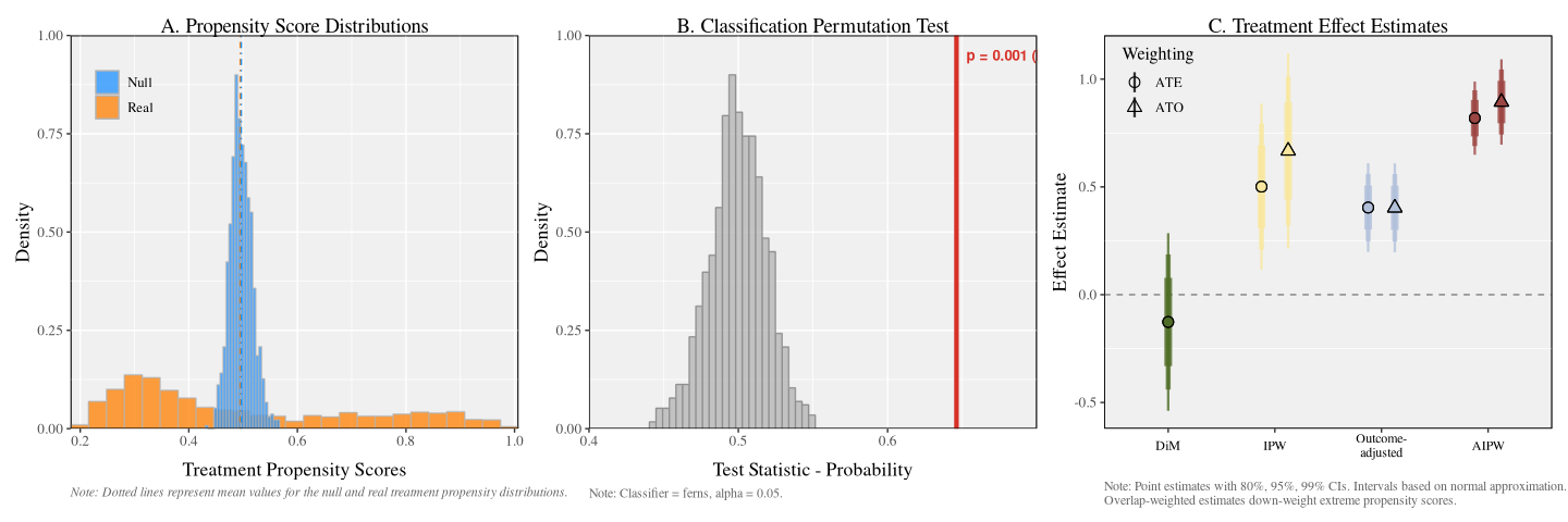
To summarize, simply execute:
b |> summary()
#>
#> ========================================================================
#>                    COVARIATE BALANCE ASSESSMENT
#> ========================================================================
#>
#> 1. SAMPLE
#> ------------------------------------------------------------------------
#>    Observations:    1000
#>    Control ('0'):  504 (50.4%)
#>    Treatment:       496 (49.6%)
#>
#> 2. CLASSIFICATION PERMUTATION TEST
#> ------------------------------------------------------------------------
#>    Classifier:          ferns
#>    Permutations:        1000
#>    Test statistic:      0.6461
#>    Null mean (SD):      0.4994 (0.0190)
#>    P-value:             0.0010
#>    Alpha:               0.05
#>    Result:              FAIL
#>
#>    Propensity scores (boosted regression forest):
#>                            Real        Null
#>    ----------------------------------------
#>    Mean:                 0.4947      0.4966
#>    SD:                   0.2207      0.0204
#>    Min:                  0.1824      0.4302
#>    Max:                  1.0077      0.5671
#>    ----------------------------------------
#>    Diff. in means:      -0.0018
#>    Ratio of SDs:        10.8183
#>
#> 3. INTERPRETATION
#> ------------------------------------------------------------------------
#>    The classification permutation test rejects the null hypothesis,
#>    indicating that treatment and control groups differ in their
#>    covariate distributions. The classifier can distinguish between
#>    groups better than random chance.
#>
#> ========================================================================
#>                    TREATMENT EFFECT ESTIMATION
#> ========================================================================
#>
#> 4. ESTIMATES
#> ------------------------------------------------------------------------
#>    Estimator                    Estimate        SE                95% CI
#>    ---------------------------------------------------------------------
#>    DiM                           -0.1265    0.1599  [ -0.4400,   0.1869]
#>    IPW                            0.5008    0.1496  [  0.2077,   0.7940]
#>    Outcome-adjusted               0.3941    0.0796  [  0.2380,   0.5501]
#>    AIPW                           0.8070    0.0661  [  0.6775,   0.9366]
#>
#>    OVERLAP WARNING: 16 observations have extreme propensity scores
#>    (< 0.05 or > 0.95). Overlap-weighted estimates down-weight these:
#>
#>    Estimator                    Estimate        SE                95% CI
#>    ---------------------------------------------------------------------
#>    IPW (OW)                       0.6671    0.1757  [  0.3227,   1.0116]
#>    Outcome-adj. (OW)              0.3931    0.0797  [  0.2368,   0.5493]
#>    AIPW (OW)                      0.8825    0.0771  [  0.7313,   1.0337]
#>
#>
#> 5. ESTIMATOR DIVERGENCE TESTS
#> ------------------------------------------------------------------------
#>    Comparison                    Difference   SE(diff)   z-stat   p-value
#>    ----------------------------------------------------------------------
#>    DiM vs IPW                       -0.6274     0.0691   -9.084    0.0000 *
#>    DiM vs Outcome-adj.              -0.5206     0.1241   -4.195    0.0000 *
#>    DiM vs AIPW                      -0.9336     0.1314   -7.106    0.0000 *
#>    IPW vs AIPW                      -0.3062     0.1197   -2.557    0.0106 *
#>    * p < 0.05
#>
#>    Significant divergences:
#>
#>    DiM vs IPW: The IPW estimate differs from the unadjusted DiM
#>    by 0.6274 units (z = -9.084, p = 0.0000), indicating that propensity
#>    reweighting accounts for this difference.
#>
#>    DiM vs Outcome-adjusted: The outcome-adjusted estimate differs from
#>    the unadjusted DiM by 0.5206 units (z = -4.195, p = 0.0000), indicating
#>    that outcome regression adjustment accounts for this difference.
#>
#>    DiM vs AIPW: The AIPW estimate differs from the unadjusted DiM
#>    by 0.9336 units (z = -7.106, p = 0.0000), reflecting the combined
#>    effect of propensity and outcome adjustment.
#>
#>    IPW vs AIPW: Adding outcome regression to propensity reweighting
#>    changes the estimate by 0.3062 units (z = -2.557, p = 0.0106),
#>    indicating that outcome modeling captures additional
#>    covariate-outcome associations beyond reweighting.
#>
#> 6. ESTIMATOR GUIDE
#> ------------------------------------------------------------------------
#>    All adjusted estimators use grf::causal_forest's AIPW framework.
#>    They differ in which nuisance models (propensity and/or outcome)
#>    are estimated vs. held at uninformative constants.
#>
#>    We present four ATE estimates as a robustness decomposition.
#>    Agreement across estimators signals robustness to modeling choices.
#>    Divergence reveals which adjustment component (propensity vs.
#>    outcome) most affects the estimate and warrants investigation.
#>
#>    Nuisance models are fit using honest, tuned boosted regression
#>    forests (grf::boosted_regression_forest; honesty = TRUE,
#>    tune.parameters = "all"); all predictions are out-of-bag.
#>    Treatment effects are estimated via grf::causal_forest
#>    and grf::average_treatment_effect (target = "all").
#>    Standard errors use the infinitesimal jackknife (IJ) influence
#>    function. DiM SEs use Neyman's separate-variance (Welch) formula.
#>    All confidence intervals use a normal approximation.
#>
#>    DiM (difference-in-means)
#>      E[Y|W=1] - E[Y|W=0]. No covariate adjustment.
#>
#>    IPW (inverse propensity weighted)
#>      W.hat = boosted-RF propensity; Y.hat = mean(Y) (constant).
#>      Isolates the effect of propensity score reweighting.
#>
#>    Outcome-adjusted (regression adjustment)
#>      W.hat = mean(W) (constant); Y.hat = boosted-RF outcome predictions.
#>      Isolates the effect of outcome regression adjustment.
#>
#>    AIPW (augmented IPW / doubly robust)
#>      Both nuisance models estimated. Consistent if either is correct.
#>
#>    Overlap-Weighted (OW) Estimates
#>      When propensity scores approach 0 or 1, AIPW estimators become
#>      unstable. Overlap-weighted estimates (Li, Morgan & Zaslavsky, 2018)
#>      target the ATE for the overlap population by down-weighting units
#>      with extreme propensity scores. Computed via
#>      grf::average_treatment_effect(target.sample = "overlap").