A unified function for covariate balance assessment and treatment effect estimation. Combines a formal balance test (via classification permutation test), visual diagnostics (propensity score distributions), and treatment effect estimates using both difference-in-means and AIPW (augmented inverse propensity weighting).
Supports both binary and multi-arm treatments. For multi-arm treatments, pairwise comparisons are made between each treatment arm and the control group.
Usage
balance(
  Y = NULL,
  W,
  X,
  alpha = 0.05,
  perm.N = 1000,
  class.method = "ferns",
  seed = 1995,
  control = NULL,
  clusters = NULL,
  blocks = NULL,
  num.trees = 2000,
  overlap.threshold = c(0.05, 0.95),
  fastcpt.args = list()
)

# S3 method for class 'balance'
print(x, ...)

# S3 method for class 'balance'
summary(object, ...)

# S3 method for class 'balance'
plot(x, which = "all", combined = TRUE, breaks = 25, ...)
Arguments
- Y
Outcome vector (numeric) or
NULL. IfNULL, treatment effect estimation (and the treatment effect plot) is skipped.- W
Treatment assignment vector. Can be binary (0/1, logical) or multi-arm (factor, character, or integer with >2 levels).
- X
Pre-treatment covariate matrix or data frame.
- alpha
Significance level for balance test. Default is 0.05.
- perm.N
Number of permutations for the balance test. Default is 1000.
- class.method
Classification method for balance test. Can be "ferns" (default), "forest", "glmnet2", "lm", "rpart", "lda", or "qda". See
fastcptfor the authoritative list and details on each backend. To use an ensemble of classifiers, passfastcpt.args = list(class.methods = c("ferns", "forest")).- seed
Random seed for reproducibility. Default is 1995.
- control
Optional. The value in
Wto use as the control group. IfNULL(default), the first factor level is used as control. A message is displayed indicating the control assumption.- clusters
Optional vector of cluster identifiers (same length as
W). When provided, permutations in the balance test shuffle treatment labels at the cluster level, and treatment effect standard errors use cluster-robust variance estimators. Treatment must be constant within each cluster.- blocks
Optional vector of block identifiers (same length as
W). When provided, permutations in the balance test are restricted to within each block.- num.trees
Number of trees used in
grf::causal_forest()for treatment effect estimation. Default is 2000.- overlap.threshold
Numeric vector of length 2 giving the lower and upper propensity score thresholds for flagging overlap issues. Default is
c(0.05, 0.95). When any propensity scores fall outside these bounds, overlap-weighted estimates are automatically computed.- fastcpt.args
A named list of additional arguments to pass to
fastcpt. For example,fastcpt.args = list(parallel = TRUE, leaveout = 0.2). You can also pass classifier-specific hyperparameters through this list, e.g.,fastcpt.args = list(classifier.args = list(num.trees = 1000))for ranger,list(classifier.args = list(ferns = 1000))for rFerns, orlist(classifier.args = list(nfolds = 10))for cv.glmnet. You can also use this to run an ensemble of classifiers:fastcpt.args = list(class.methods = c("ferns", "forest")).- x
A balance result object.
- ...
Additional arguments (currently unused).
- object
A balance result object (for summary method).
- which
Character vector specifying which plots to create. Options are "pscores", "null_dist", "effects", or "all".
- combined
Logical. If TRUE, displays all three plots in a combined panel. Default is TRUE.
- breaks
Number of breaks for histograms. Default is 25.
Value
A list of class "balance" containing:
- balance_test
Results from fastcpt including p-value and propensity scores. For multi-arm, a named list with one entry per treatment arm.
- dim
Difference-in-means estimate with standard error and confidence interval (only if
Yis provided). For multi-arm, a named list.- ipw
IPW estimate using propensity scores from the boosted regression forest, with SE and CI (only if
Yis provided). For multi-arm, a named list.- aipw
AIPW (doubly robust) estimate from causal forest (with propensity weighting) with standard error and CI (only if
Yis provided). For multi-arm, a named list.- oadj
Outcome-adjusted estimate from causal forest (no propensity weighting) with SE and CI (only if
Yis provided). For multi-arm, a named list.- passed
Logical indicating whether the balance test passed. For multi-arm, a named logical vector.
- alpha
The significance level used.
- cf
The fitted causal_forest object(s) for advanced users (only if
Yis provided). For multi-arm, a named list.- imp.predictors
Variable importance scores from the propensity model, computed via
vip. For multi-arm, a named list.- control
The control level used.
- arms
Character vector of treatment arm names (excluding control).
- multiarm
Logical indicating whether this is a multi-arm analysis.
- overlap_flag
Logical indicating whether overlap issues were detected.
- overlap
Overlap-weighted estimates (if
overlap_flagisTRUE).- n_extreme
Number of observations with extreme propensity scores.
- pscores_real
Propensity scores from the real treatment assignment.
- pscores_null
Propensity scores from a permuted treatment assignment.
- n
Number of observations.
- n_treated
Number of treated units (binary case).
- n_control
Number of control units (binary case).
- n_per_arm
Named vector of sample sizes per arm (multi-arm case).
- clusters
Cluster identifiers (if provided).
- blocks
Block identifiers (if provided).
- ate_cov
Covariance matrix of ATE estimates (used in divergence tests).
Examples
# \donttest{
# Generate example data (binary treatment)
n <- 500
p <- 10
X <- matrix(rnorm(n * p), n, p)
W <- rbinom(n, 1, 0.5)
Y <- W * 0.5 + X[,1] * 0.3 + rnorm(n)
# Run complete balance assessment
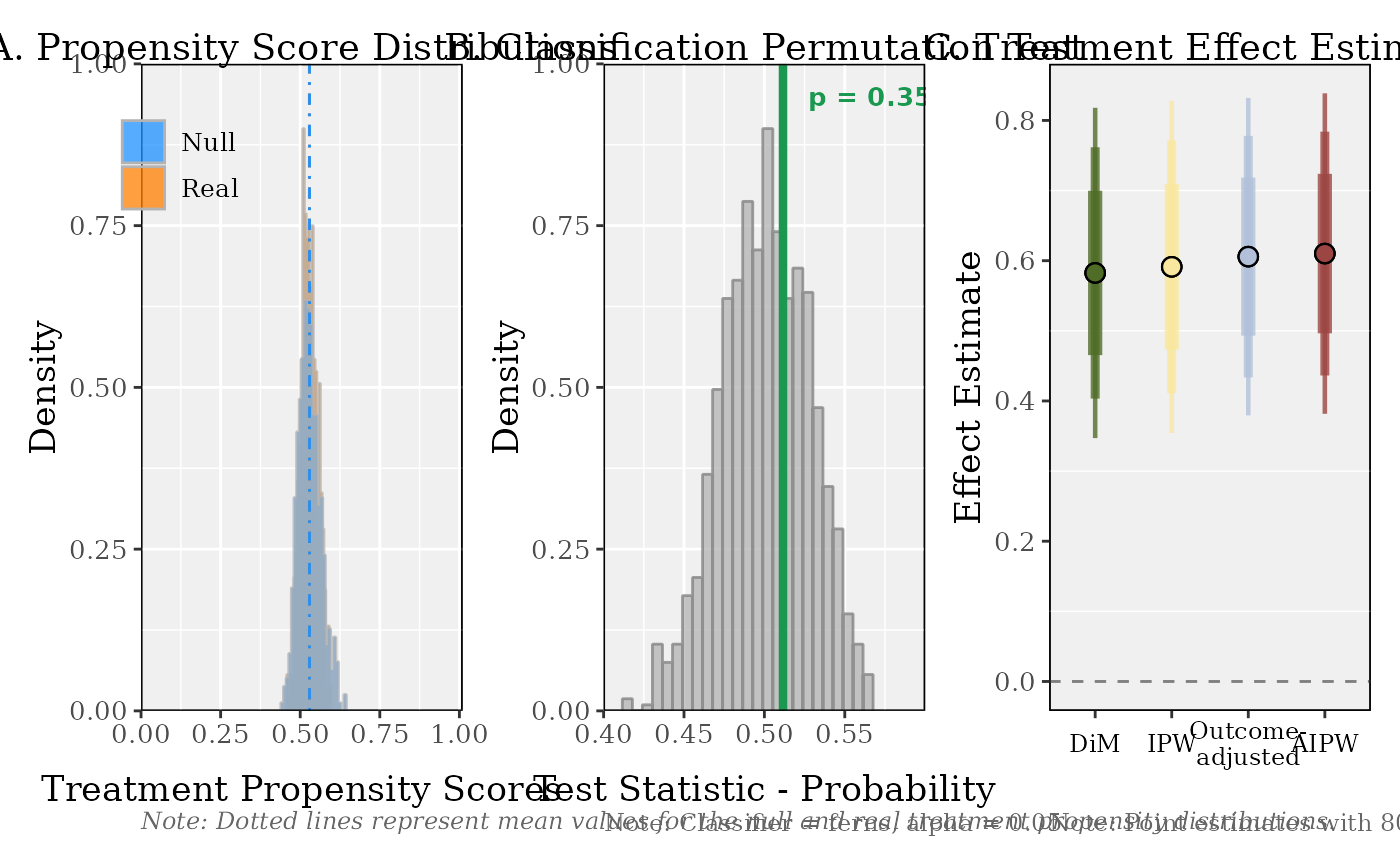
result <- balance(Y, W, X)
result
#>
#> Balance Assessment
#> ------------------------------------------------------------
#> Control: '0'
#> Balance: p = 0.3586 [PASS]
#>
#> Treatment Effect Estimates
#> ------------------------------------------------------------
#> DiM: 0.5825 (SE: 0.0914)
#> IPW: 0.5913 (SE: 0.0920)
#> Outcome-adjusted: 0.6058 (SE: 0.0879)
#> AIPW: 0.6102 (SE: 0.0887)
#>
#> Use summary() for full details, plot() to visualize.
#>
summary(result)
#>
#> ========================================================================
#> COVARIATE BALANCE ASSESSMENT
#> ========================================================================
#>
#> 1. SAMPLE
#> ------------------------------------------------------------------------
#> Observations: 500
#> Control ('0'): 236 (47.2%)
#> Treatment: 264 (52.8%)
#>
#> 2. CLASSIFICATION PERMUTATION TEST
#> ------------------------------------------------------------------------
#> Classifier: ferns
#> Permutations: 1000
#> Test statistic: 0.5116
#> Null mean (SD): 0.5009 (0.0275)
#> P-value: 0.3586
#> Alpha: 0.05
#> Result: PASS
#>
#> Propensity scores (boosted regression forest):
#> Real Null
#> ----------------------------------------
#> Mean: 0.5286 0.5292
#> SD: 0.0262 0.0350
#> Min: 0.4575 0.4390
#> Max: 0.5970 0.6451
#> ----------------------------------------
#> Diff. in means: -0.0005
#> Ratio of SDs: 0.7474
#>
#> 3. INTERPRETATION
#> ------------------------------------------------------------------------
#> The classification permutation test does not reject the null
#> hypothesis that treatment and control groups are drawn from the
#> same covariate distribution. The classifier cannot distinguish
#> between groups better than chance.
#>
#> ========================================================================
#> TREATMENT EFFECT ESTIMATION
#> ========================================================================
#>
#> 4. ESTIMATES
#> ------------------------------------------------------------------------
#> Estimator Estimate SE 95% CI
#> ---------------------------------------------------------------------
#> DiM 0.5825 0.0914 [ 0.4034, 0.7617]
#> IPW 0.5913 0.0920 [ 0.4109, 0.7716]
#> Outcome-adjusted 0.6058 0.0879 [ 0.4336, 0.7780]
#> AIPW 0.6102 0.0887 [ 0.4363, 0.7841]
#>
#> 5. ESTIMATOR DIVERGENCE TESTS
#> ------------------------------------------------------------------------
#> Comparison Difference SE(diff) z-stat p-value
#> ----------------------------------------------------------------------
#> DiM vs IPW -0.0087 0.0051 -1.707 0.0879
#> DiM vs Outcome-adj. -0.0233 0.0197 -1.178 0.2386
#> DiM vs AIPW -0.0276 0.0209 -1.324 0.1855
#> IPW vs AIPW -0.0189 0.0200 -0.946 0.3443
#>
#> All four estimators agree closely, indicating the ATE estimate is
#> robust to the choice of nuisance model specification.
#>
#> 6. ESTIMATOR GUIDE
#> ------------------------------------------------------------------------
#> All adjusted estimators use grf::causal_forest's AIPW framework.
#> They differ in which nuisance models (propensity and/or outcome)
#> are estimated vs. held at uninformative constants.
#>
#> We present four ATE estimates as a robustness decomposition.
#> Agreement across estimators signals robustness to modeling choices.
#> Divergence reveals which adjustment component (propensity vs.
#> outcome) most affects the estimate and warrants investigation.
#>
#> Nuisance models are fit using honest, tuned boosted regression
#> forests (grf::boosted_regression_forest; honesty = TRUE,
#> tune.parameters = "all"); all predictions are out-of-bag.
#> Treatment effects are estimated via grf::causal_forest
#> and grf::average_treatment_effect (target = "all").
#> Standard errors use the infinitesimal jackknife (IJ) influence
#> function. DiM SEs use Neyman's separate-variance (Welch) formula.
#> All confidence intervals use a normal approximation.
#>
#> DiM (difference-in-means)
#> E[Y|W=1] - E[Y|W=0]. No covariate adjustment.
#>
#> IPW (inverse propensity weighted)
#> W.hat = boosted-RF propensity; Y.hat = mean(Y) (constant).
#> Isolates the effect of propensity score reweighting.
#>
#> Outcome-adjusted (regression adjustment)
#> W.hat = mean(W) (constant); Y.hat = boosted-RF outcome predictions.
#> Isolates the effect of outcome regression adjustment.
#>
#> AIPW (augmented IPW / doubly robust)
#> Both nuisance models estimated. Consistent if either is correct.
#>
plot(result)
 # Multi-arm example
W_multi <- sample(c("Control", "Treatment A", "Treatment B"), n, replace = TRUE)
Y_multi <- (W_multi == "Treatment A") * 0.3 + (W_multi == "Treatment B") * 0.6 + rnorm(n)
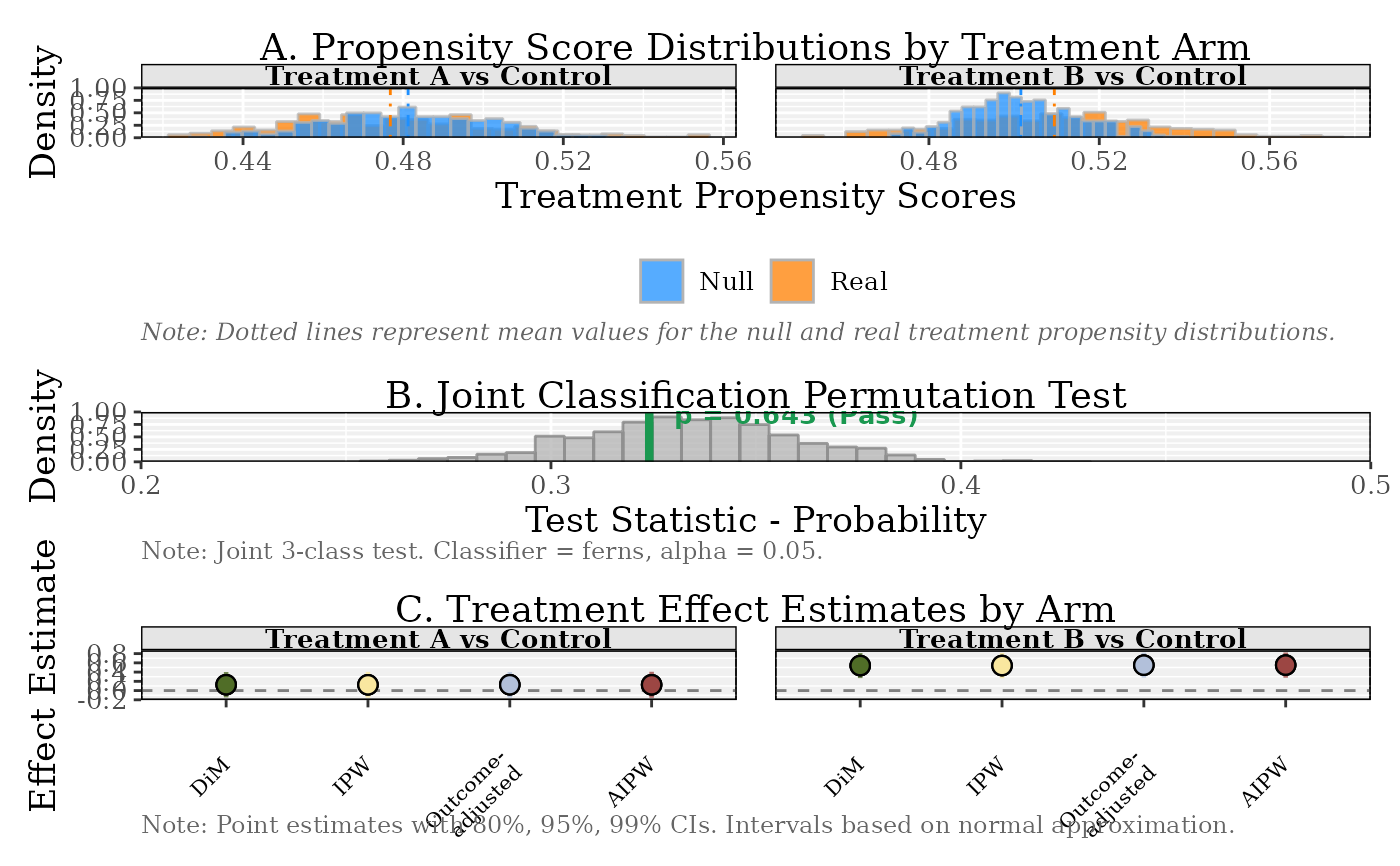
result_multi <- balance(Y_multi, W_multi, X, control = "Control")
#> Using 'Control' as control group.
plot(result_multi)
# Multi-arm example
W_multi <- sample(c("Control", "Treatment A", "Treatment B"), n, replace = TRUE)
Y_multi <- (W_multi == "Treatment A") * 0.3 + (W_multi == "Treatment B") * 0.6 + rnorm(n)
result_multi <- balance(Y_multi, W_multi, X, control = "Control")
#> Using 'Control' as control group.
plot(result_multi)
 # }
# }