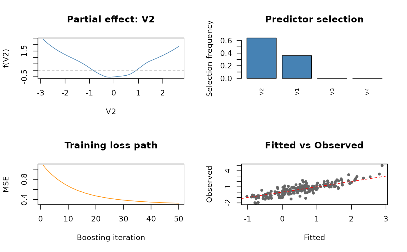
Produces a 4-panel diagnostic display for a fitted component-wise P-spline boosting model:
Usage
# S3 method for class 'bgam'
plot(x, ...)
Arguments
- x
An object of class
"bgam", as returned bybgam().- ...
Currently ignored.
Details
Partial effect curve \(\hat{f}_{j^*}(x_{j^*})\) for the top predictor by selection frequency, plotted over a fine grid covering the training range.
Selection-frequency bar chart for all predictors (capped at 20 bars), sorted descending. Use this panel to identify which predictors drive the model.
Training loss path (MSE for gaussian, mean deviance per observation for binomial) vs boosting iteration. A red dashed vertical line marks
mstop_optwhenautotune = TRUE.Fitted vs Observed (gaussian) or fitted-probability box plots by class (binomial).
The function works in headless (non-interactive) mode without error.
References
Buehlmann, P. and Yu, B. (2003). Boosting with the L2 loss: Regression and classification. Journal of the American Statistical Association, 98(462):324–339. doi:10.1198/016214503000125
Hofner, B., Mayr, A., Robinzonov, N. and Schmid, M. (2014). Model-based boosting in R: A hands-on tutorial using the R package mboost. Computational Statistics, 29(1–2):3–35. doi:10.1007/s00180-012-0382-5